Sequence Training for Neural Networks in Matlab

I had 77 pairs of sequences and sequence responses in Matlab. I had two cell arrays, sequences and responses, of dimension 77×1. Each cell held a 10×10,000 array. I created options, layers, and hyperparamaters, and executed

[net, info] = trainNetwork(sequences, responses, layers, options);

The network trained. Things worked.

I got more data, hundreds of pairs. I could still train the network, but I was rapidily coming to the memory limit on my HPC. I wanted to use datastores.

S(cripts) 1
save(‘sequences.mat’,’sequences’);
save(‘responses.mat’,’responses’);

S2
AData = fileDatastore(‘sequences.mat’,’Readfcn’,’@load’);
BData = fileDatastore(‘responses.mat’,’Readfcn’,’@load’);
CData = combine(AData, BData);

… %stuff
[net, info] = trainNetwork(CData, layers, options);

Error using trainNetwork (line 184)
Invalid training data. Predictors must be a N-by-1 cell array of sequences, where N is the number of sequences. All sequences
must have the same feature dimension and at least one time step.

Error in S1 (line ##)
[net, info] = trainNetwork(CData, layers, options);

Or in English, it did not work.

Using preview, I got this:

ans =

1×2 cell array

{1×1 struct} {1×1 struct}

First, the load function creatues a struct. I needed a de-struct-ing function.

Now, I got this.

preview(CData)

ans =

1×2 cell array

{259×1 cell} {259×1 cell}

Second, the combine function creats another cell array, meaning I had a 1×2 cell array (CData), each cell holding a 200×1 cell array (AData and BData), but those were holding lesser datastores.

The solution to the latter was saving each cell as an individual file with one vairable per file, that variable being the 10×10,000 array, NOT A CELL.

S3
%file manip, mkdir, addpath, etc.

for n=1:length(sequences)
sequence1 = sequences{n,1};
response1 = responses{n,1};
save(strcat(‘sequences’,string(n),’,mat’),’sequence1′);
save(strcat(‘responses’,string(n),’,mat’),’sequence1′);
end

AND THEN running S4

%file manip, preprocessing, etc.

getVarFromStruct = @(strct,varName) strct.(varName);
xds = fileDatastore(“sequences*.mat”,”ReadFcn”,@(fname) getVarFromStruct(load(fname),”sequence1″),”FileExtensions”,”.mat”);
yds = fileDatastore(“responses*.mat”,”ReadFcn”,@(fname) getVarFromStruct(load(fname),”response1″),”FileExtensions”,”.mat”);

%options, layers, hp, etc.

[net, info] = trainNetwork(CData, layers, options);

And it worked.

In the preview of CData up there, it creates 2 cell arrays OF CELLS. TrainNetwork doesn’t want cells; it wants data. So the extra layer of cells caused all those errors.

That took me weeks, and someone else had to explain it.
Convergents to rad(2)

I didn’t find anything too interesting.

I’m pretty sure it’s spelled Convergence, but hey, maybe it’s branding.

Q gets to n=21 before hitting the limit. I guess I could look for a most efficient upgrade path for manual buying.
N=zeros(1,100);
D=zeros(1,100);
Q=zeros(1,100);

N(1)=1;
N(2)=3;

D(1)=1;
D(2)=2;

Q(1)=abs(sqrt(2)-N(1)/D(1))^-1;
Q(2)=abs(sqrt(2)-N(2)/D(2))^-1;

for index=3:100
N(index)=2*N(index-1)+N(index-2);
D(index)=2*D(index-1)+D(index-2);
Q(index)=abs(sqrt(2)-N(index)/D(index))^-1;
end

%some random numbers

c1=25;
c2coeff=4;
n=4;

qdot_base=qdotfunc(c1,c2coeff,n,Q);
qdot_C1=qdotfunc(c1+2,c2coeff,n,Q); %note the +2
qdot_C2=qdotfunc(c1,c2coeff+1,n,Q);
qdot_n=qdotfunc(c1,c2coeff,n+1,Q);

%=================================================
%new file
function [qdot] = qdotfunc(c1, c2coeff, n, Q)

m=n*c2coeff;
c2=2^c2coeff;

qdot=c1*c2*Q(m);

%====================================================

I dunno. Am I missing anything?

Matlabbery

Weierstrass Sine Product, qdot simulator.

%Matthew Miller
%v_4
%2/8/22
%Calculates max qdot for a range of n and c1 values
%to do more I’d have to optimize a time-dependent progression
%I may do it later

%pdot = q1*q2*q
%qdot = m3Factor * s_n(chi)/sin(chi)
%s_n(chi) = chi * PI(k=1:n)(1-(chi/(k*pi))^2)

%==========================================================================
%start fresh

clear all

%==========================================================================
%human entry

%set number of purchases
steps = 1000;

%since the maximum number of purchases of each variable is all of the
%purchases, these can be set to steps
nDimension = steps;
c1Dimension = steps;

%not sure what to do with these yet
q1=1;
q2=1;
c2=1;

m1=4; %Milestone upgrade 1 level (0, 1, 2, 3, or 4)
m2=1; %Milestone upgrade 2 level (0 or 1)
m3=3; %Milestone upgrade 3 level (0, 1, 2, or 3)

%==========================================================================
%prelim calculations

nIndex=1:nDimension; %X axis
c1Index=1:c1Dimension; %Y axis

m1Factor = q1^(1+0.01*m1); %precalculate
m2Factor = c2^m2; %precalculate
m3Factor = 3^m3; %precalculate

chi = zeros(nDimension,c1Dimension); %preallocate for speed
sinterm = zeros(nDimension,c1Dimension); %preallocate for speed
s_n = zeros(nDimension,c1Dimension); %preallocate for speed
qdot = zeros(nDimension,c1Dimension); %preallocate for speed

%==========================================================================
%generate variables
%Normally I’d do all these with functions, but that’s harder to read

%blah blah blah arrays begin at 1 so I’m ignoring c1(0)=0

stepLength = 50;
basePower = 1;
offset = 1;

power=basePower;
c1steps=1;

c1(1)=offset;

for index = 2:c1Dimension
c1(index) = c1(index-1)+power;
c1steps=c1steps+1;
if c1steps > stepLength
power=power*2;
c1steps=1;
end
end

%chi
for n_index=1:nDimension %X
for c1_index=1:c1Dimension %Y
chi(n_index,c1_index) = pi.*c1(c1_index).*nIndex(n_index)./(c1(c1_index)+nIndex(n_index)/m3Factor)+1; %x=n, y=c1
end
end

%sin(chi)
for n_index=1:nDimension %X
for c1_index=1:c1Dimension %Y
sinterm(n_index,c1_index) = sin(chi(n_index,c1_index));
end
end

%s_n(chi)
for n_index=1:nDimension %X
for c1_index=1:c1Dimension %Y
s_n(n_index,c1_index) = chi(n_index,c1_index);
s_nk(1)=chi(n_index,c1_index)*(1-(chi(n_index,c1_index)/(1*pi))^2);
if n_index>1
for k = 2:n_index %Big Pi
s_nk(k)=s_nk(k-1)*(1-(chi(n_index,c1_index)/(k*pi))^2);
end
end
s_n(n_index,c1_index)=s_nk(end);
end
end

%qdot(chi)
for n_index=1:nDimension %X
for c1_index=1:c1Dimension %Y
qdot(n_index,c1_index)=m2Factor*s_n(n_index,c1_index)/sinterm(n_index,c1_index);
end
end

[M,I] = max(qdot(:));
[n_max, c1_max] = ind2sub(size(qdot),I); %Maximum values
qdot(n_max,c1_max);

%========================================================================================
%plotter
%========================================================================================

clear rows cols

maxSteps = steps;
minSteps = 1;
for stepsIndex=minSteps:maxSteps

nRange=stepsIndex;
c1Range=stepsIndex;

C=max(qdot(1:nRange,1:c1Range));
D=max(C);
[rows(stepsIndex), cols(stepsIndex)] = find(qdot(1:nRange, 1:c1Range) == D);

end

figure(1)
plot(rows, cols)
title(‘Peak Qdot’)
xlabel(‘n’)
ylabel(‘c1’)

EI&WSP

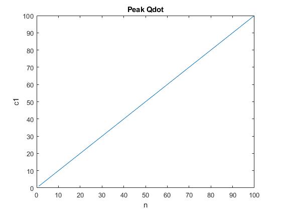
Without cost, the best purchase works out to be linear. There’s no cool backstepping or ommissions worth chasing.

I’m hunting around for typos, but it seems to match up with the game results pretty carefully. Perhaps including a cost function, there will be a way to beat the autobuyer.

Matlab

I never noticed something in 10+ years.

For arrays in the variable viewer pane, Matlab displays the X values on the vertical axis and the Y values on the horizontal axis.

Create a nxn array. Label it A(n1, n2).

I think of n1 as X and n2 as Y. I think of the array as being A(x, y).

But when I view that array in Matlab, the x values will be indexed vertically on the left side and the y values are indexed horizontally on the top. If I open A(n1, n2) in the variable viewer pane, n1 (what I think of as x) is the vertical dimension and n2 (y) is the horizontal dimension. n1 is across the left, and n2 the top. (Plots are different)

That could be better.

Exponential Idle and the Weierstrass Sine Product

Dangit, Conic. Stop dropping updates late at night. I have to sleep.

Within the first 20 options of n and c1, the peak is n=18, c1=19.

Within the first 500, n=484 c1=311.

Matlabbery:


%Matthew Miller
%1/16/22
%Calculates max qdot for a range of n and c1 values
%to do more I’d have to optimize a time-dependent progression
%I may do that later

%pdot = q1*q2*q
%qdot = m3Factor * s_n(chi)/sin(chi)
%s_n(chi) = chi * PI(k=1:n)(1-(chi/(k*pi))^2)

%==========================================================================
%start fresh

clear c1 n chi sinterm s_n M I qdot n_max c1_max

%==========================================================================
%human entry

dimension = 36;

%not sure what to do with these yet
q1=1;
q2=1;
c1=1;
c2=1;
c3=1;

m1=0; %Milestone upgrade 1 level (0, 1, 2, 3, or 4)
m2=0; %Milestone upgrade 2 level (0 or 1)
m3=1; %Milestone upgrade 3 level (0, 1, 2, or 3)

%==========================================================================
%prelim calculations

n=1:dimension; %X axis
c1=1:dimension; %Y axis

m1Factor = q1^(1+0.01*m1); %precalculate
m2Factor = c3^m2; %precalculate
m3Factor = 3^m3; %precalculate

chi = zeros(dimension,dimension); %preallocate for speed
sinterm = zeros(dimension,dimension); %preallocate for speed
s_n = zeros(dimension,dimension); %preallocate for speed
qdot = zeros(dimension,dimension); %preallocate for speed

%==========================================================================
%generate variables
%Normally I’d do all these with functions, but that’s harder to read

%chi
for n_index=1:length(n) %X
for c1_index=1:length(c1) %Y
chi(n_index,c1_index) = pi.*c1(c1_index).*n(n_index)./(c1(c1_index)+n(n_index)./m3Factor)+1; %x=n, y=c1
end
end

%sin(chi)
for n_index=1:length(n) %X
for c1_index=1:length(c1) %Y
sinterm(n_index,c1_index) = sin(chi(n_index,c1_index));
end
end

%s_n(chi)
for n_index=1:length(n) %X
for c1_index=1:length(c1) %Y
s_n(n_index,c1_index) = chi(n_index,c1_index);
for k = 1:length(n_index) %Big Pi
s_n(n_index,c1_index)=s_n(n_index,c1_index)*(1-(chi(n_index,c1_index)/(k*pi))^2);
end
end
end

%qdot(chi)
for n_index=1:length(n) %X
for c1_index=1:length(c1) %Y
qdot(n_index,c1_index)=s_n(n_index,c1_index)/sinterm(n_index,c1_index);
end
end

%==========================================================================
%find max qdot

[M,I] = max(qdot(:));
[n_max, c1_max] = ind2sub(size(qdot),I); %Maximum values

%waterfall(qdot(1:10,1:10));


I bounce between writing concise, readable, and optimized code. Text file here.

Edit: Newer txt file here. Also: plotter.

The Monty Hall Problem

Suppose you’re on a game show, and you’re given the choice of three doors: Behind one door is a car; behind the others, goats. You pick a door, say No. 1, and the host, who knows what’s behind the doors, opens another door, say No. 3, which has a goat. He then says to you, “Do you want to pick door No. 2?” Is it to your advantage to switch your choice?

The official answer is…switch. You double your odds of being right by switching.

This has led to some vigorous debate.

I read it in Jo Craven McGinty’s final column, instantly decided all of these idiots were wrong, and did some Matlabbery.

The idiots were right. You double your chances of being right by switching.

BUT WHY?

Let’s go chronologically.

Step 1:

The car is somewhere, the goats are somewhere. These positions are fixed. No car-goat switching shenanigans take place.

Step 2:

You pick a door.

You have 1/3 chance, 33.33….% chance of getting it right.

THAT IS IT. THIS GUESS IS DONE. THE CHANCE OF YOUR INITIAL GUESS BEING CORRECT IS FINISHED, COMPLETED, SET, and NOT CHANGING.

Step 3:

The host looks behind the doors and picks one with a goat. This door is opened. You, the contestant, can see the hosts door opened to reveal a goat.

Step 4:

You may change your guess to the other door.

This is where the magic happens.

That initial guess is locked at 1/3 chance, 33% (and hereafter I’m neglecting the .333… repeating). It cannot change. But there’s still an outstanding 2/3 chance of finding the car. The car has to be somewhere. Since you already know, for a fact, that there’s only 1/3 chance of your first guess being correct, and you know there’s 0% chance of it being behind the host’s door (remember, the host opened that door. You can see the goat), the remaining chance has to be behind the other door.

So switching has to improve your odds.

But it just doesn’t feel right, does it? Why not?

Because you think about things after they’re done.

If you picked your first guess after the host opened a door, then the two options would be 50/50, what feels right. But that’s not what happens. The first guess is made and locked BEFORE the host opens the door, so it has to be fixed at 1/3. The host doesn’t move the cars and goats around after opening a door, so the odds don’t reset.

Matlab: MontyHall
(Change ending from .txt to .m or copy and paste)

I suppose you also might want a goat. I’m neglecting that.

Logistics Map

Want to see something weird?

The Logistics Map is the iterative function: xn+1 = a*xn*(1-xn) where xn is some number between zero and 1, non-inclusive, alpha is a number between zero and 4, and xn+1 is the number you get when you do the math on xn.

So pick an x value arbitrarily: 0.6. x1 = 0.6

Pick alpha arbitrarily: 3.56995. alpha = 3.56995.

x2 = 3.56995 *0.6 * (1-0.6) =3.56995*0.6*0.4= 0.854388

That’s xn+1. xn in this case is x1. Think of xn+1 as being the next x. So you have a first x, 0.6, and the next x is 0.854388, and the next x is 0.438041158193768.

I picked the alpha because the numbers are highly chaotic and don’t go outside (0,1). The parenthesis means 0 and 1 are not included.

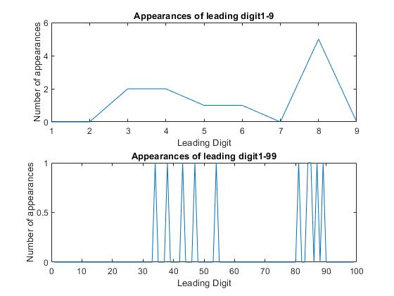
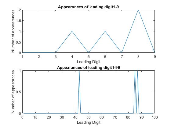
Then, for funsies, I bin the leading digits. So x1 is 6, x2 is 8, x3 is 4, etc. Zeros are never leading digits, so if a number was 0.0002, the leading digit would be 2. For extra funsies, I do the same for the first two digits below. (The images are named after the number of times I go through the function, so they’re 10s +1)

This is the plot of the first 11 values:

Okay, so what?

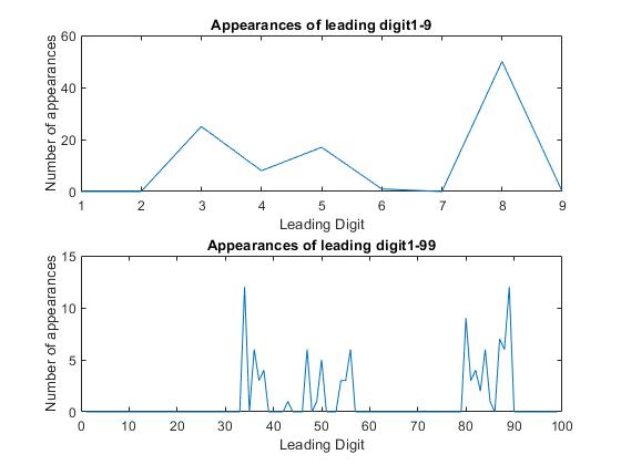
This is the first 101 values:

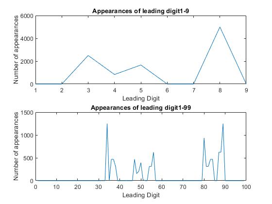
This is the first 10,001:

The shape doesn’t change. Oh, it squiggles a little. Here’s the first 4:

Other than resolution improvements, the shape remains basically the same for the leading digit graph. Does it do that for the double leading digit graph?